
One of my hobbies is miniature painting, it’s something I did a long time ago and found myself getting back into a year or so back. Now I am nowhere near an expert on this, but do like to work on techniques and ideas I see online and on the dreaded Youtube. That’s where I got an idea about the colour theory.
If you have ever done any art work, you will probably have heard of colour theory and the famous colour wheels. Well I saw a few videos on it and though that it might be helpful to me in choosing colours and working out the best colour for contrast colours and also maybe to help make sense of my expanding set of Vallejo Game Colours.
What I found was that although there were plenty of talks about using the wheel, there didn’t seem to be any mapping of the paint colours that you can buy to it.
Sounds like a simple task I thought. How wrong could I be…
Well the first stage was to get the paint colours and their RGB values. Eventually after hunting I found a repository with very helpful paint cross matches at: this site and in particular for my use I the Vallejo Game Colour page. Now this does have the names and RGB values, so a quick bit of web-scraping later and I have an excel sheet with the name, hex code and decoded RGB values.
Next stage how to create a Colour wheel, looking on Wikipedia shows many different types, but the basic seems to be just a ring of colour, or with a graduation towards the centre. Which can be either to Black or to White. I wanted a simple way of generating this and fell back onto a simple file creation of a BMP file using python. I am sure there are better ways, but for what I needed this was fine, and lets me work on the files quickly.
This gave me:

Note I converted this to JPG both for size (but also as WordPress would not let me upload the raw JPG).
This seems to match the colour wheel I have seen so I think I got this right. For those interested, this is created by having and outer ring of 100% Red, Green and Blue for 120° each and then with a fade to 0 over the next 60° in each direction. i.e. there is some green in 240° of the circle, and the same for each of the Red, and Blue elements. These all then linearly fade to 0 in the centre.
I did a few experiments with fading to white in the middle and even a hybrid wheel with black in the centre and white on the outside with a colour saturation a the mid point. This looks quite nice to be honest, but in the end it didn’t really help me as you will see.
So next, how to map the colours onto the wheel. This should be the easy part. Well this is where I realised why nobody seems to have done it.
I started to look at the actual RGB values of the paints, and with only a few exceptions I saw that there where always some Red, some Blue and some Green.
NOTE: This seems obvious now, but I didn’t seem anybody mention this in the theory posts. Probably I just missed it.
So what does this mean for the mapping. Well basically if there are only 2 of the primary colours in the paint then the paint can be mapped directly on the wheel, but as soon as there are elements of all three then the colour is no longer a pure colour but is a de-saturated colour, a good example of this is flesh tones, these are generally reddish yellows, so would be primarily Red, with Green as the secondary colour. But there is also a significant amount of Blue. If they where even of course you would get a pure grey (or white if all at maximum).
Not wanting to give up, I concluded that the colour would be a mix of the Primary and secondary colours and an saturation offset. So to work this out I preprocessed all the RGB values to subtract the lowest colour value from all of them.
For example Moon Yellow has RGB values of 255, 207 and 7 . I converted this to 248, 200, 0 and a saturation value of 7.
With Just the two colours and the offset I was able to map the colours onto the wheel, this gives the following Image (again as JPG):

Having produced the colour wheel with the Vallejo Game Colour paints shown, this shows that there is a lot of colours all close together nearer the black end (i.e. the middle on this chart). Now this is also of course made worse by the process I did to get to Primary and secondary colours (i.e. remove the tertiary colour evenly).
So to try to make these more visible, I tried an alternative view of the data as a linear chart with black at the bottom and full saturation colours at the top. Clearly this does not help with the original colour wheel for opposites, but does produce the chart below:

Now clearly as this is not circular, I have had to make a break at one point and for this I chose the purple (-60° on the wheel) as this appears to have the least colours available and hence is the easiest to split.
What surprises me here is that this shows there is a gap around pure green as well as the purple, I was not expecting this, but now looking at the circular chart you can also see it there with the angle between fluorescent green and scorpion green being blank right to the black white centre point.
Note. Anyone else think Star Trek The Motion Picture when they saw this.
Next given these are based on the colour when saturation is taken into account, the overall colours appear darker than reality, so the next step to me was to create a similar chart but showing the actual brightness rather than the colour match.
For this I think a grey chart with just colour on the outside would work best, so let’s see what that looks like:

NOTE: I have changed the brightness offset arrow and the location circle to a sample of the actual colour. I found this easier to understand, and it does show the issue of the RGB to wheel mapping, as there is some cases where there are 2 different colour sample very close together.
For example around 1/3 of the way out on the 7 o’clock position you will see the overlap of Heavy Blue and Cold Grey which are different, but mainly due to their relative saturations.

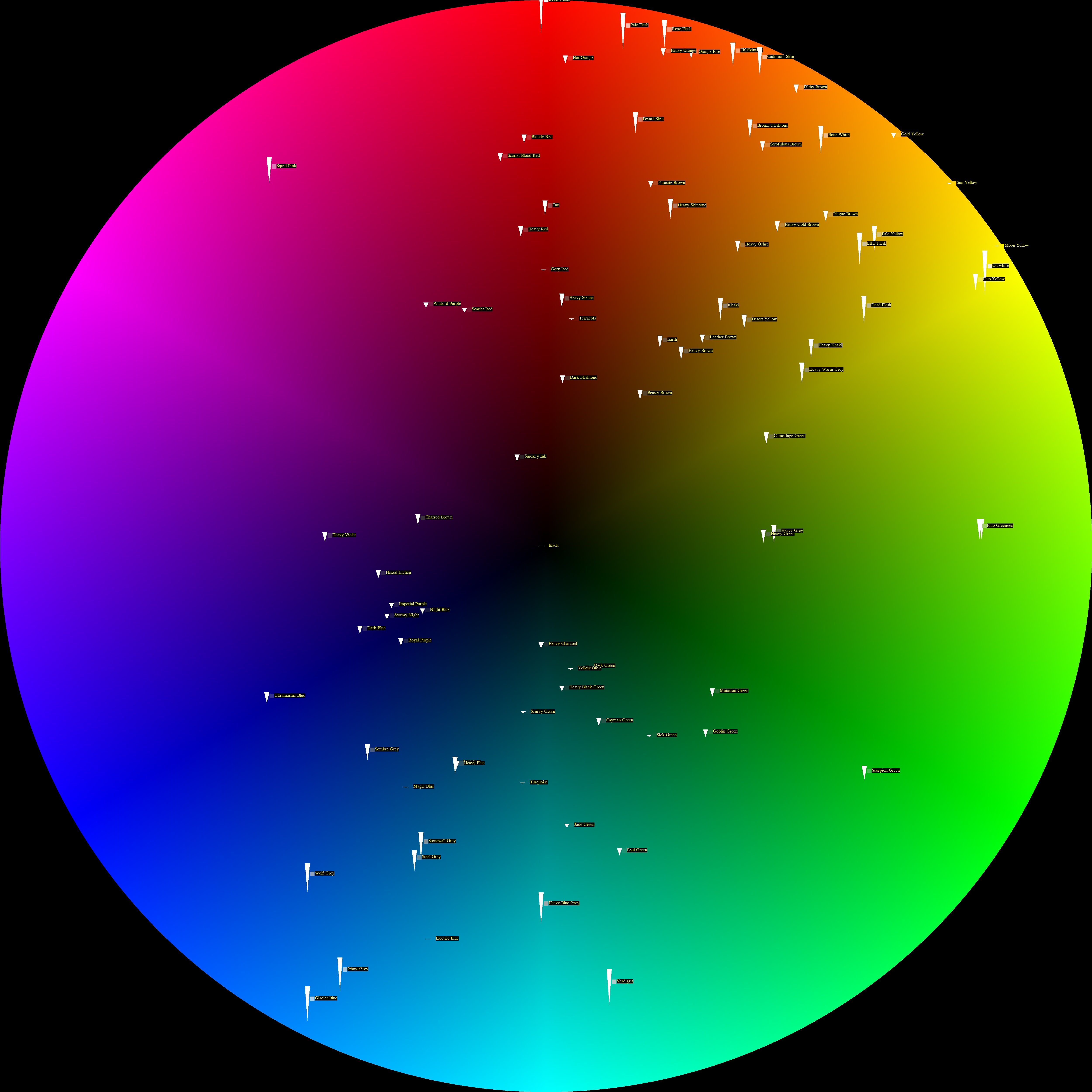
Further for clarity I went back to the colour wheel as the background but the relative brightness as the position on the axis, with a down arrow showing the relative desaturation of colour, this along with the sample square seems to give the best view from my perspective.
I have also updated the test rendering to give a solid black box for the text as this makes it easier to read.
The final chart as it stands is below:

A higher resolution (and hence smaller text version) can be found here.
If you find this helpful, then let me know, or better if you have any ideas how to improve this or how best to use it then please send me a comment.